Data Assimilation Primer
Before beginning the tutorial, it will be useful to have a basic understanding of paleoclimate data assimilation (DA). On this page, we’ll provide an overview of DA and review some common tasks for these analyses. DASH is often used to implement Kalman filters, so we’ll also briefly review this method. (We’ll also describe DASH’s DA algorithms in greater detail later in the tutorial).
Overview
In the broadest terms, data assimilation combines climate model output (\(\mathrm{X_p}\)) with proxy records (\(\mathrm{Y}\)) to create reconstruct a set of target climate variables (\(\mathrm{X_a}\)). Formally, we can write this as:
The reconstruction proceeds by updating climate variables in the climate model output (\(\mathrm{X_p}\)) to more closely match the proxy records (\(\mathrm{Y}\)). The updated climate variables (\(\mathrm{X_a}\)), sometimes called the (a)nalysis, form the reconstruction.
Two of the most common paleoclimate DA techniques - the Kalman filter, and the particle filter - can be expressed as Bayesian filters. In this context, information from the climate proxy records \(\mathrm{Y}\) is used to update estimates of state parameters (climate variables) \(\mathrm{X}\). Because of this, we will often refer to the initial climate model output \(\mathrm{X_p}\) as the prior, and the updated output \(\mathrm{X_a}\) as the posterior.
State Vectors
In general, the climate model output is organized into state vectors. These consist of spatiotemporal climate model output reshaped into a vector of data values:
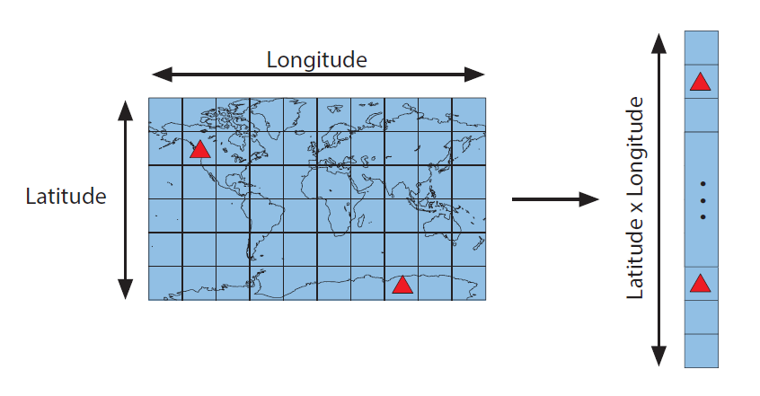
Figure 1: A spatial field is reshaped into a state vector. (Red triangles represent the locations of proxy sites).
There is no strict definition for the contents of a state vector, but they typically include data for one or more climate variables at a set of spatial points. A state vector might also contain a trajectory of successive points in time; for example, individual months of the year or a number of successive years following an event of interest. Essentially, a state vector serves as a possible description of the climate system for some period of time.
Ensembles
The DASH toolbox focuses on ensemble DA methods, which rely on state vector ensembles. A state vector ensemble is a collection of multiple state vectors organized in a matrix:
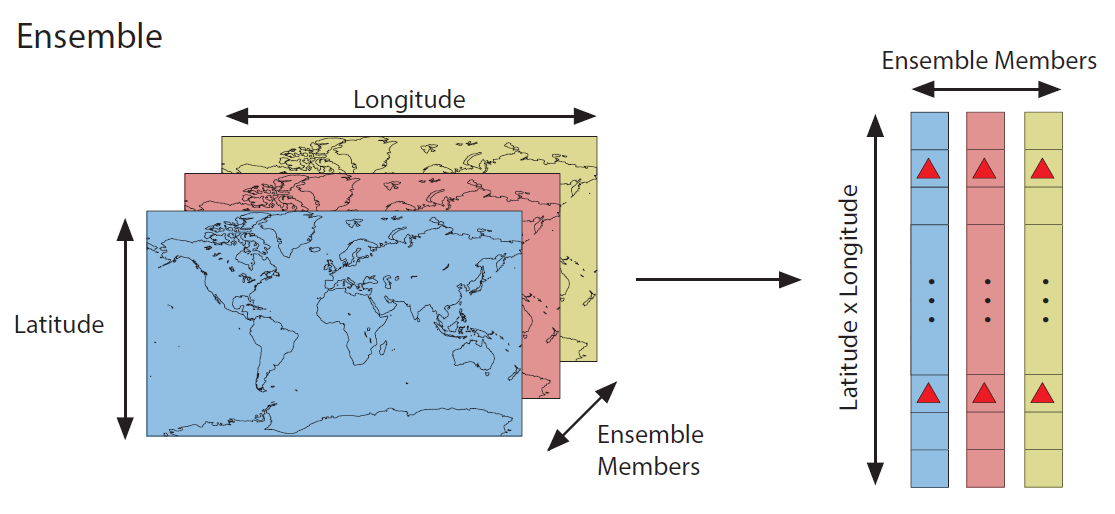
Figure 2: Multiple state vectors are grouped together into an ensemble.
An ensemble provides an empirical distribution of possible climate states. For paleoclimate DA, ensemble members are often selected from different points in time, different members of a model ensemble, or both.
In a typical DA algorithm, the state vectors in an ensemble are compared to a set of proxy record values in a given time step. Essentially, the method compares potential descriptions of the climate system (taken from a climate model) to proxy values from the real past climate record. The similarity of each state vector to the proxy records is then informs the final reconstruction.
Proxy Estimates
In order to compare state vectors with a set of proxy record values, DA methods must transfer the state vectors and proxy records into a common unit space. This is accomplished by applying proxy forward models to relevant climate variables stored in each state vector. Applying a forward model to a state vector produces a value in the same units as the corresponding proxy record, which allows direct comparison of the state vector and observed proxy value.
Typically, DA methods will run a forward model to estimate each proxy record for each state vector in an ensemble. The collective outputs are referred to as the proxy estimates (\(\mathrm{\hat{Y}}\)):
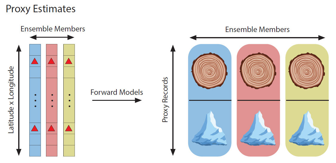
Figure 3: Proxy estimates for a state vector ensemble. Forward models are used to estimate a tree-ring record and an ice-core record for each state vector in the ensemble.
Ultimately, these proxy estimates allow comparison of each state vector with the real proxy records. The difference between the proxy estimates and the real records is known as the innovation:
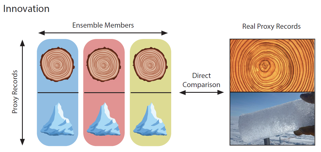
Figure 4: Proxy estimates are compared directly to the real proxy records. The difference between the two is known as the innovation.
Written formally:
The innovation is then used to update the prior ensemble (\(\mathrm{X_p}\)) so that it more closely resembles the observed proxy records.
Proxy Uncertainties
In addition to proxy innovations, the DA methods in DASH also consider proxy uncertainties (\(\mathrm{R}\)) when comparing state vector to proxy records. More formally:
In this way, proxy records with high uncertainties are given less weight in the reconstruction. In classical assimilation frameworks \(\mathrm{R}\) is usually derived from the uncertainty inherent in measuring an observed quantity (for example, the uncertainty of width measurements in a tree-ring chronology). However, in nearly all paleoclimate applications, measurement uncertainties are small compared to
The uncertainties of the proxy forward models, and
Uncertainties from non-climatic noise in the proxy records
Thus, in paleoclimate DA, the proxy uncertainties \(\mathrm{R}\) must account for proxy noise and forward model errors, as well as any covariance between different proxy uncertainties.
Kalman Filter
When using a Kalman filter, the update equation is:
The equation indicates that the innovation is weighted by the Kalman Gain matrix (K) in order to compute an update for each state vector. The Kalman Gain weighting considers multiple factors including:
The covariance of the proxy estimates (\(\mathrm{\hat{Y}}\)) with the target climate variables (\(\mathrm{X_p}\))
The covariance of the proxy estimates (\(\mathrm{\hat{Y}}\)) with each other, and
The proxy uncertainties (\(\mathrm{R}\))
Written formally, the Kalman Gain matrix is given by:
You won’t need to remember this equation for the tutorial, but it can be useful to understand how the assimilation works.
Applying the Kalman Gain to the innovation produces a set of updates. Applying these updates to the prior ensemble (\(\mathrm{X_p}\)) produces an updated (posterior) ensemble (\(\mathrm{X_a}\)), such that the climate states (state vectors) in \(\mathrm{X_a}\) more closely resemble those recorded by the real proxy records.
Typically, we use the mean of this updated ensemble as the final reconstruction. However, the ensemble nature of the posterior is also useful because the distribution of climate variables across \(\mathrm{X_a}\) can help quantify uncertainty in the reconstruction.